

Lorem ipsum dolor sit amet, consectetur adipiscing elit. Suspendisse varius enim in eros elementum tristique. Duis cursus, mi quis viverra ornare, eros dolor interdum nulla, ut commodo diam libero vitae erat. Aenean faucibus nibh et justo cursus id rutrum lorem imperdiet. Nunc ut sem vitae risus tristique posuere.
Lorem ipsum dolor sit amet, consectetur adipiscing elit. Suspendisse varius enim in eros elementum tristique. Duis cursus, mi quis viverra ornare, eros dolor interdum nulla
Key Takeaways
- Principle: A thermocouple measures the temperature difference between the measuring junction and the cold junction. Heating the measuring junction raises the voltage, while heating the cold junction lowers it.
- Probe uncertainty: Even with perfect electronics, a Type K probe can deviate by 1.5 °C (Class 1) or 2.5 °C (Class 2). That is why you calibrate the probe together with the electronics.
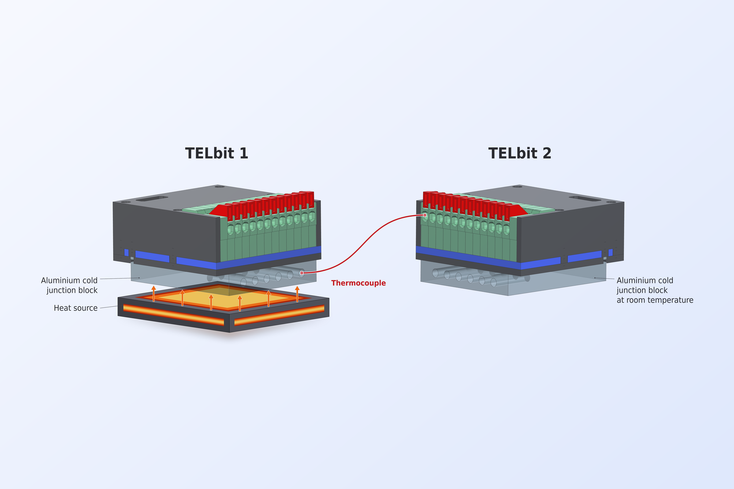
- Method: Two TELbits with an aluminium terminal block and an internal sensor (0.1 °C) as the reference. There are three tests: heating the measuring junction, heating the cold junction, and a zero check for the offset.
- Range: Up to about 100 °C. Above that, a correction is extrapolation and needs verification.
In this first part, we explain the theory behind our thermocouple calibration procedure. We use two of our latest TELbit sensors, designed specifically for thermocouples. The aluminium terminal block on one unit provides a temperature reference for the other. This lets us investigate what happens to the measured voltage when we heat the measuring junction and what happens when we heat the terminals.
The curves in this article show the response we expect. We will expand this post with experimental data and compare our measured voltages with those predictions.
1. How does a thermocouple generate a voltage, and how accurate is the measurement?
When we talk about thermocouple accuracy, we often start with the electronics. How accurately does the TELbit measure the voltage at its input? With a precise readout, the thermocouple itself can be the largest source of uncertainty. At a given pair of junction temperatures, an individual probe can produce a voltage that differs from the reference curve for its type.
Consider a Type K thermocouple. Its sensitivity, sometimes called gain, tells us how much the voltage changes per degree of warming at the measuring junction while the cold junction stays at a fixed temperature. From 20 to 30°C, the nominal sensitivity averages 40.5 µV/°C. From 80 to 90°C, it averages 41.5 µV/°C. The slope of the reference curve changes with temperature.
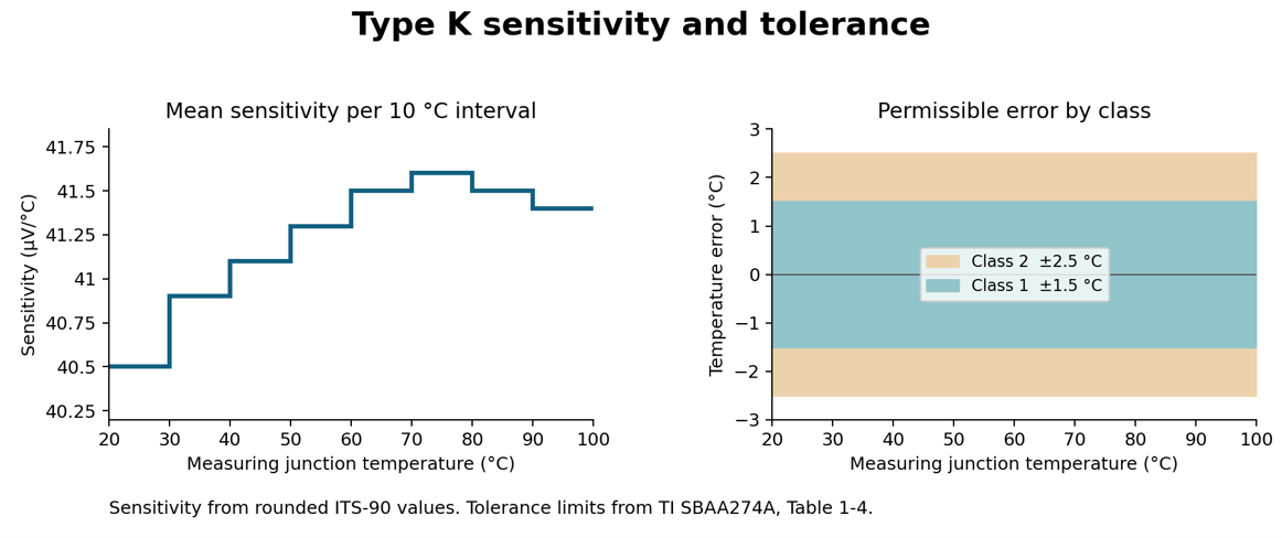
Tolerance tells us how far an individual probe may deviate from the reference curve, expressed in degrees. Between 20 and 100°C, the Type K limits are ±1.5°C for Class 1 and ±2.5°C for Class 2. Even if the electronics measure the voltage exactly, a Class 2 probe can therefore introduce a larger temperature error. Calibrating the probe together with the electronics lets us determine the deviation of the particular probe we use.
A thermocouple consists of two dissimilar metal conductors joined at the measuring junction. Their other ends connect to the TELbit at two terminals held at the same temperature. Together, these connections form the cold junction. Through the Seebeck effect, a temperature gradient along each conductor generates a voltage. The voltage measured across the terminals is the difference between the two conductors’ contributions.
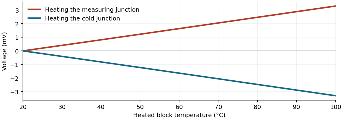
For a homogeneous thermocouple, the measured voltage is E(Thot) − E(Tcold) where E is the reference voltage function for that thermocouple type. This gives us two responses to investigate. Heating the measuring junction alone increases the Type K voltage. Heating the cold junction alone decreases it.
2. What do we need for calibration?
We need a reference that tells us the temperature of the measuring junction and a heat source that lets us vary that temperature in a controlled way.
The TELbit’s aluminium terminal block sits flush against the printed circuit board (PCB) at the cold junction. An internal sensor measures the local temperature with a specified accuracy of 0.1 °C. The block also has holes that accept a thermocouple’s measuring junction, bringing the measuring junction, cold junction and internal sensor close together.
Aluminium conducts heat well, and we use thermal paste to fill small air gaps at the contact surfaces. Once the assembly reaches thermal equilibrium, we can reasonably assume that the block, the PCB at the cold junction and the inserted measuring junction are at practically the same temperature. That assumption allows us to use the internal sensor as the reference for the measuring junction in the block.
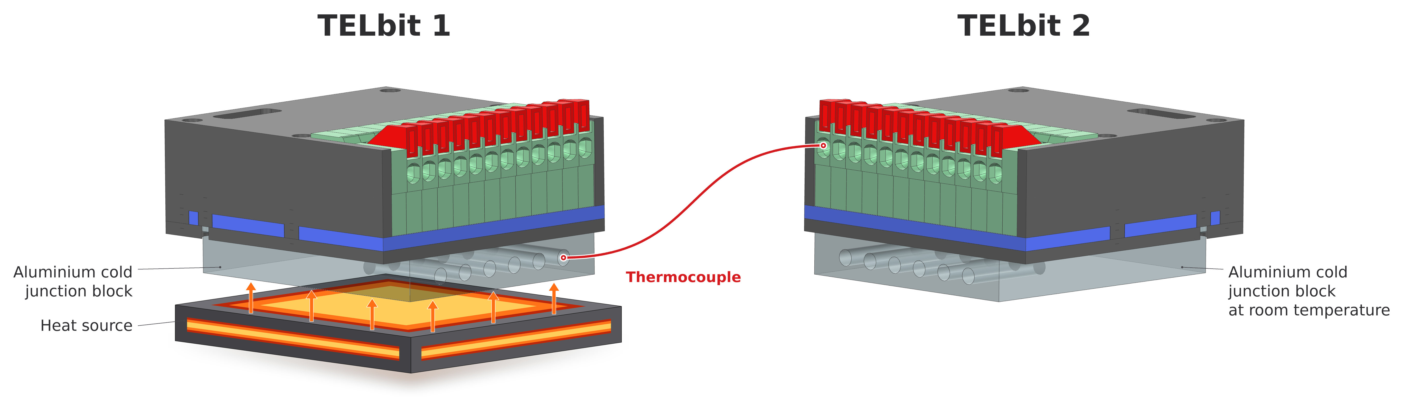
We apply heat to the underside of one block, for example with the heated bed of a 3D printer. The other block stay sat room temperature. After each heating step, we wait for both sensor readings to stabilise. The difference between the readings gives us the temperature difference applied across the thermocouple.
3. Two response curves and a zero check
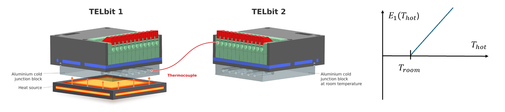
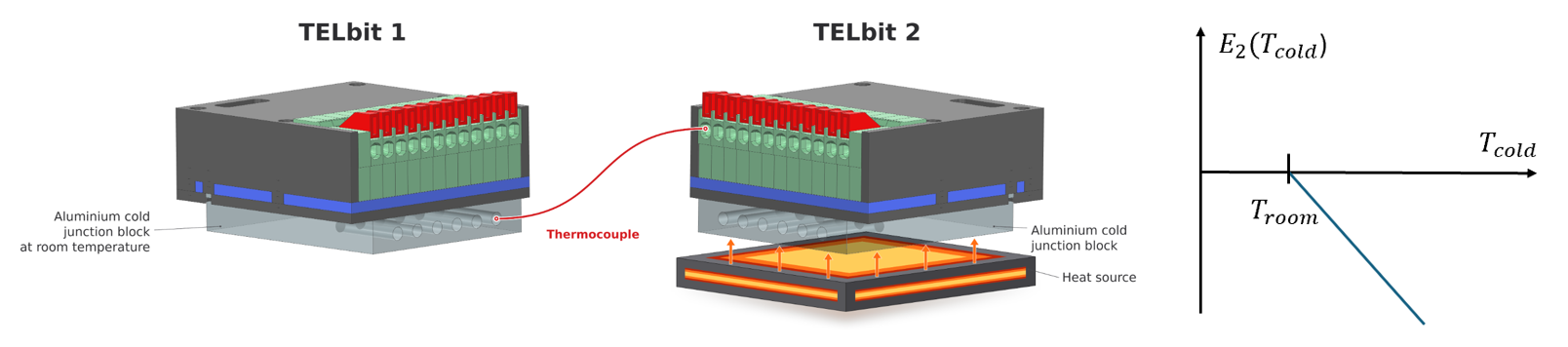
For all three experiments, we use the same thermocouple on the same input channel of TELbit 2. At each stable temperature step, we record both block temperatures and the raw voltage before old-junction compensation. The sketches show the expected response, starting at room temperature.
Experiment 1 · Heating the measuring junction
The measuring junction sits in the block on TELbit 1, which we heat from below. The cold junction on TELbit 2 stays at room temperature. As the measuring junction warms up, the voltage at the TELbit 2 input rises.
Experiment 2 · Heating the cold junction
We move the heat source to TELbit 2. The measuring junction stays at room temperature in the block on TELbit 1. As the cold junction warms up, the raw voltage falls. After cold-junction compensation, the calculated measuring-junction temperature should continue to track the temperature of block 1.
Experiment 3 · Checking the zero offset
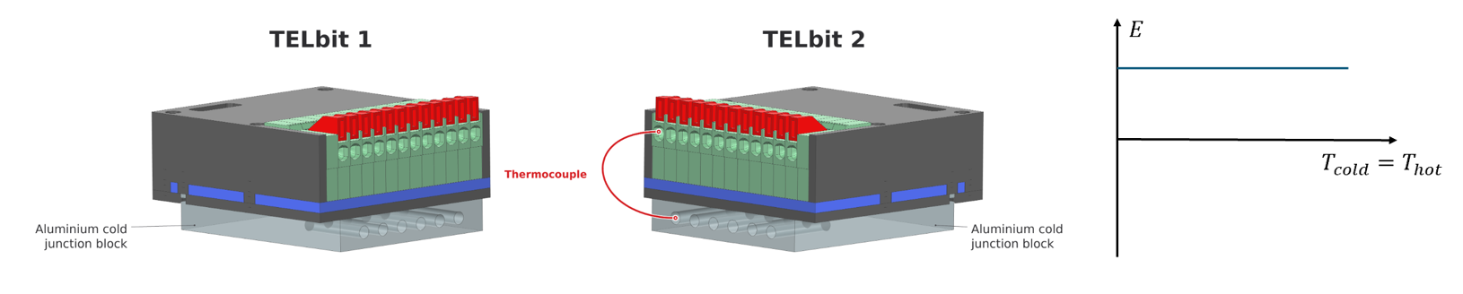
We insert the measuring junction into the aluminium block on TELbit 2, keeping the thermocouple connected to the same channel. Once the block is thermally stable, the two junctions are at the same temperature, so the expected thermocouple voltage is 0 mV. Any residual voltage is the offset of the measurement chain at that operating point. Repeating the check at several block temperatures tests whether the offset stays constant, as illustrated by the horizontal line.
How far does this calibration extend?
Our cold-junction sensor covers 0 to 100°C. With a heated bed and the second block at room temperature, we can test from room temperature upwards. Points nearer 0 °C require cooling. Above 100°C, the Type K reference curve still applies, but extending a correction determined for an individual probe amounts to extrapolation. Calibration at higher temperatures requires a suitable reference and measurements in that range.
What this means for a reliable measurement
At Forcebit, we design both the sensor and the tools to test the complete measurement chain. The Seebeck effect tells us how the voltage should respond when either junction warms up, and the zero check lets us measure any residual offset. With this setup, we can calibrate up to approximately 100 °C. Once we have collected the experimental data, we can use the deviation from the standard Type K reference curve to estimate a correction at higher temperatures. This extends the range over which we can estimate temperature. Above 100 °C, that correction is an extrapolation, and its accuracy must be verified against a reference at those higher temperatures.
Sources: Texas Instruments, A Basic Guide to Thermocouple Measurements (SBAA274A), Table 1-4 and Figure 1-4, www.ti.com/lit/pdf/sbaa274. NIST ITS-90 Thermocouple Database, Type K, its90.nist.gov.